- Financial calculator
- Spreadsheet, like Excel
Excel functions
First of all, we will look at the three functions we need to use (Do note that most other spreadsheet programs use the exact same functions). 1. PMT (Rate, NPer,PV, FV, Type): Total payment (principle and interest) payable for that compounding period 2. PPMT (Rate, Per, NPer, PV, FV, Type): Principle payable for that compounding period 3. IPMT (Rate, Per, NPer, PV, FV, Type): Interest payable for that compounding period So what is each of the variables in the parenthesis? Note that the ones in italics are optional.- Rate (Required): Nominal interest rate for that compounding period
- NPer (Required): Total number of compounding periods
- PV (Required): Present value of the loan
- FV: Loan amount outstanding after all payments have been made. If this variable is omitted, Excel will assume the default value of 0.
- Type: The timing of the payment. It can be either 0 or1. If this variable is omitted, Excel will assume the default value of 0.
|
Value |
Explanation |
| 0 | Payments are due at the end of the period. (default) |
| 1 | Payments are due at the beginning of the period. |
- Per: The particular compounding period for which you want to find the interest or principle payable.
Creating the amortisation schedule
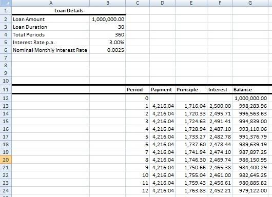
Rest, or the compounding period, is the frequency in which the outstanding loan amount is calculated. For the purpose of this exercise, we will assume the most common case of a monthly-rest loan. Example: Rest = Monthly Loan Amount = $ 1,000,000 Loan Duration = 30 years Interest Rate = 3% per annum for the first year 5% per annum thereafter We enter these information into the Excel sheet, as below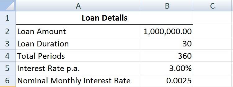
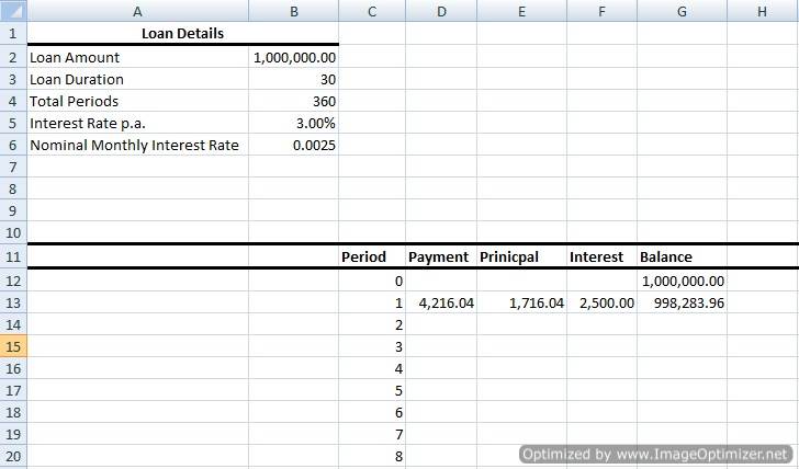
Table 1
|
Cell |
Enter |
|
G12 |
=B2 |
|
D13 |
=PMT(B$6,B$4,-B$2) |
|
E13 |
=PPMT(B$6,C13,B$4,-B$2) |
|
F13 |
=IPMT(B$6,C13,B$4,-B$2) |
|
G13 |
=G12-E13 |
 So after finding the amorisation schedule for the first year, what about the second year? We set up a new amortization schedule with different values, as below.
 The loan amount becomes the outstanding balance at the end of the first year (i.e. Period 12), which is $ 979,122.
The remaining loan duration is 29 years; while the annual interest rate becomes the 2nd year rate.
To find the amortisation schedule for Period 0 and 1 we enter the exact same syntax as in Table 1. Since there is no change in interest rate from the 2nd year onwards, we can drag the formulas down until the end of the loan, which is the 348th period.
The loan amount becomes the outstanding balance at the end of the first year (i.e. Period 12), which is $ 979,122.
The remaining loan duration is 29 years; while the annual interest rate becomes the 2nd year rate.
To find the amortisation schedule for Period 0 and 1 we enter the exact same syntax as in Table 1. Since there is no change in interest rate from the 2nd year onwards, we can drag the formulas down until the end of the loan, which is the 348th period.
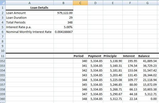 At the 348th period, the loan is completely paid off, so the balance (outstanding loan) is $0.
The amortisation schedule worksheet, with the formulas, can be DOWNLOADED HERE. To calculate the amortization schedule for your loan, all you have to do is key the relevant information in the 'Loan Details'. And presto! You can see the amortisation schedule for Period 0 and 1. Pull and drag the formulas down to find the values for the rest of the periods.
At the 348th period, the loan is completely paid off, so the balance (outstanding loan) is $0.
The amortisation schedule worksheet, with the formulas, can be DOWNLOADED HERE. To calculate the amortization schedule for your loan, all you have to do is key the relevant information in the 'Loan Details'. And presto! You can see the amortisation schedule for Period 0 and 1. Pull and drag the formulas down to find the values for the rest of the periods.
About Property Buyer http://www.PropertyBuyer.com.sg/mortgage We are a research-focused Singapore mortgage consultancy which helps you compare Singapore home loans either for new loans or refinancing. We use loan reports from Singapore's best loan analysis system (exclusive to us) at http://www.icompareloan.com/consultant/ to serve our customers. Our services are completely FREE to you as the banks pay us a referral fee upon loan disbursement. SMS: (65) 9782 8606 Email: loans@PropertyBuyer.com.sg